Direction finding with compact Volumetric Acoustic Sensor (cVAS)#
The following script demonstrates different methods to estimate the direction of sound sources using a comapct volumetric acoustic sensor. Sound sources are simulated to provide the opportunity to assess the quality of the direction estimations.
note to myself: jupyter nbconvert cVAS_direction.ipynb –to html
Loading libraries#
First, some basic libraries are imported and general parameter defined.
import numpy as np
import matplotlib.pyplot as plt
import scipy.signal as signal

import bioacoustic_tools as bat
plt.rc('font', size=15)
#
print(help(bat))
Help on module bioacoustic_tools:

NAME
    bioacoustic_tools

DESCRIPTION
    # %% [markdown]
    # # bioacoustic tools

FUNCTIONS
    B_path(hd, sd, bd)
        bottom reflected path

    D_path(hd, sd)
        direct path

    S_path(hd, sd)
        surface reflected path

    array_delay(S, ho, sv=1500, fs=None)
        estimate delays using direction vector
        S direction vector
        ho hydrophone locations
        fs sampling frequency

    array_init(ro, type)
        contruct volimetric array of hydrophones
        ro   : radius of bounding sphere
        type : configuration ("tetahedron","octahedron","cube")

    array_setup(ho, iar=-1)
        generate vector of hydrophone pairs
        ho  : hydrophone vectors
        iar : selected sub array (-1: all pairs)

    array_timeseries(yy, DS, noise)
        delay signal according to array geometry
        (use fractional delay with sinc function)
        yy      : time series
        DS      : delay vector [samples]
        noise   : noise variance

    beamForm(yy, DS)
        delay signal according to array geometry
        (use fractional delay with sinc function)

    brownNoise(f, fo)
        brown noise (1/f**2)

    cosd(x)
        cosine of degrees

    directionFinding(xx, DI, hsel, fs, nw=None, nfft=None, nh=None, method=None)
        estimates the direction of a sound source of array recordings
        parameters
            xx: multi-dimensional time series
            DI: hydrophone array mapping function
            fs: sampling frequency
            nw: size of processing window, defautls to 256
            nfft: fft size (if needed) defaults to window size
            nh: number of positive taps (if needed, e.g hilbert transform)
            method: processing method
                'TDOA_0'    : uses local maxima of whole tim series
                'TDOA_fast' : uses time series maxima (hilbert transform)
                'TDOA'      : uses fft based cross-correlation
                'Phase'     : uses local phase differences
                'STFT'      : uses spectrogram
                'XCORR'     : uses spectrogram to cross correlate (no overlap-add)

         returns:
            Azx:   Azimuth
            Elx:   Elevation
            t:     time axis
            f:     frequency axis (if applicable)
        #

    direction_TDOA(ss, DI, hsel, nd=256)
        estimate time delay-based direction angles using cross-correlation

    direction_TDOA_0(zz, DI, hsel)
        use time differences of temporal maxima

    direction_TDOA_fast(ss, DI, hsel, nd=256)
        estimate direction using temporal maxima

    direction_intensity(xx, DI, hsel, fs, nw, nfft)
        estimated intensity based direction angles

    direction_xcorr_stft(ss, fs, nw, nover, nfft, DI, hsel, nh)
        estimate direction using stfs-based spectrogram

    dirextion_phaseShift(ss, hsel, DI, nh=None)
        estimate phase-based direction angles

    estimate_TDOA(ss, DI, hsel, nd=256)
        estimate time delay-based direction components
        process all data in small chunks

    estimate_TDOA_0(zz, DI, hsel)
        use time differences of temporal maxima

    estimate_TDOA_fast(ss, DI, hsel, nd=256)
        estimate directional direction components using temporal maxima

    estimate_intensity(xx, DI, hsel, fs, nw, nfft)
        estimated intensity based direction components

    estimate_phaseShift(ss, hsel, DI, nh=None)
        estimate phase-based direction components

    estimate_xcorr_stft(ss, fs, nw, nover, nfft, DI, hsel, nh)
        extimate cross-correlation using stfs-based spectrogram

    fft_filt(b, x, zi=None, nh=0)
        Filter a one-dimensional array with an FIR filter

        Filter a data sequence, `x`, using a FIR filter given in `b`.
        Filtering uses the overlap-add method converting both `x` and `b`
        into frequency domain first.  The FFT size is determined as the
        next higher power of 2 of twice the length of `b`.

        Parameters
        ----------
        b : one-dimensional numpy array
            The impulse response of the filter
        x : one-dimensional numpy array
            Signal to be filtered
        zi : one-dimensional numpy array, optional
            Initial condition of the filter, but in reality just the
            runout of the previous computation.  If `zi` is None or not
            given, then zero initial state is assumed.
        nh : time shift of result (group delay)

        Returns
        -------
        y : array
            The output of the digital filter.
        zf : array, optional
            If `zi` is None, this is not returned, otherwise, `zf` holds the
            final filter delay values.

    genNoise(N, fs, fo=0, method=None)
        generate colored noise
        N       : number of samples
        fs      : sampling frequency
        fo      : lower cut-off frequency
        method  : noise color method
                    pinkNoise(f)
                    brownNoise(f)
                    shipNoise(f,fo)

    hilbert_filt(ss, nh)
        filter timeseries using hilbert response (complex valued )
        ss is data to be filtered
        nh is number if (positive) coefficients of hilbert response

    lfm(f1, f2, t2, fs)
        LFM from f1 Hz to f2 Hz over t2 s, with fs sampling frequency

    matched_filt(xx, ss)
        matched filter
        xx is signal for replica
        ss is data to be filtered

    pinkNoise(f, fo)
        ping noise (1/f)

    quadInt(uu, imx, nd1)
        three point quardatic interpolation
        to find location and value of interpolated maxima
        uu  : time series
        imx : index of maxima
        nd1 : reference sample (to be subtracted from nd1)

    quadInt1(C, infft, dn)
        simple quadratic estimate interpolated maxima
        limit location of maxima to infft +- (dn-1)

    shipNoise(f, fo)
        ship noise

    signal_direction(az, el)
        estimate direction using arrival angles
        az  : azimuth angle
        el  : elevation angle

    signal_directionFromGeometry(az, dx, dy)
        estimate direction using distance, depth geometry
        dx  : horizontal distance
        dy  : vertical separation
        az  : azimuth angle

    signal_path(dx, dy, az, ho, sv)
        estimate delays using distance, depth geometry
        dx  : horizontal distance
        dy  : vertical separation
        az  : azimuth angle
        ho  : hydrophone locations

    simulate_multiPath(hd, sd, dx, bd, az, ho, sv, type)
        Simulate multi-path
        hd  : hydrophone depth
        sd  : source depth
        dx  : horizontal distance (hydrophone-source)
        az  : azimuth angle
        ho  : hydrophone locations
        type: type of arrival {'D','S','B'}

    sind(x)
        Sine of degrees

    sinfm(fc, fm, fa, t2, fs)
        Sinusoid with fc Hz center, fm Hz modulation frequency

    stack(x)
        stack time series

    tonal(fs, ax, fx)
        generate tonal from frequency
        e.g. generate 5 s LFM from 1 to 10 kHz and 96 kHz sampling
          xx=tonal(96000,1,lfm(1000,10000,5,96000))
        e.g. generate 2 s sinusoidal fm: 3 oscillations/s from 1 to 3 kHz and 96 kHz sampling
          xx=tonal(96000,1,sinfm(2000,1000,3,2,96000))

    xcorr_fft(xx, hsel, method=None)
        FFT-based cross-correlation

FILE
    c:\users\zimme\documents\bioacoustics\bioacoustic_tools.py


None
# cVAS hydrophones
ro=0.040 # m
ho=bat.array_init(ro,'octahedron')
DI,D,L,hsel=bat.array_setup(ho,0)   # chose smallest nested array (iar=0)
print(ho)
print(0.75/L,'kHz')
[[ 4.00000000e-02  0.00000000e+00 -2.82842712e-02]
 [-2.00000000e-02  3.46410162e-02 -2.82842712e-02]
 [-2.00000000e-02 -3.46410162e-02 -2.82842712e-02]
 [ 2.00000000e-02  3.46410162e-02  2.82842712e-02]
 [-4.00000000e-02  4.89858720e-18  2.82842712e-02]
 [ 2.00000000e-02 -3.46410162e-02  2.82842712e-02]]
[10.82531755 10.82531755 10.82531755 10.82531755 10.82531755 10.82531755
 10.82531755 10.82531755 10.82531755 10.82531755 10.82531755 10.82531755] kHz
Simulation of cVAS sound reception from a deep source emitting linear frequency modulated (LFM) signal.#
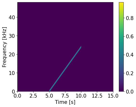
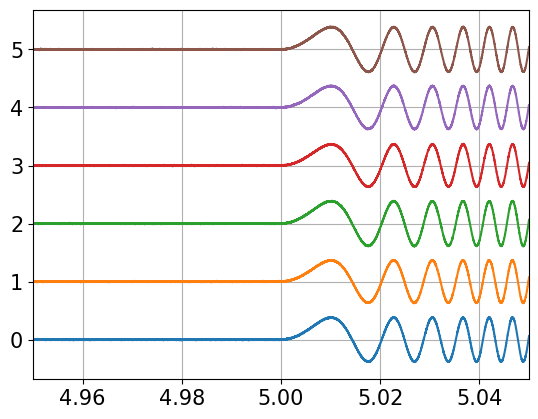
The hydrophone measurements are simulated. Here a deep sound source emitting a 5 s LFM signal covering frequencies fro 0 to 24 kHz. The signal was choosen to cover twice the expected maximal bandwidth for coherent processing. As sampling frequency 96 kHz was choosen, to have multiple samples at the upper boundary of the LFM signal.
fs=96000
f1=1
f2=24000
t2=5
sso=bat.tonal(fs,1,bat.lfm(f1,f2,t2,fs))
tt=np.arange(sso.shape[0])/fs
ss=np.concatenate((np.zeros(t2*fs),sso,np.zeros(t2*fs)))
ts=np.arange(ss.shape[0])/fs

nw=256
f,t,Q= signal.stft(ss,fs=fs,nperseg=nw,noverlap=nw//2,nfft=2*nw)
#
ext=[t[0],t[-1],f[0]/1000,f[-1]/1000]
plt.imshow(np.abs(Q),aspect='auto',origin='lower',extent=ext)
plt.colorbar()
plt.xlabel('Time [s]')
plt.ylabel('Frequency [kHz]')
plt.show()
#simulate deep source
az=135*np.pi/180
bd=900 # bottom depth m
hd=500 # hydrophone depth m
sd=800 # source depth m
dx=100 # source distance m

sv=1500
Tx,el,rx=bat.simulate_multiPath(hd,sd,dx,bd,az,ho,sv,'D')    # Tx s relative to array center
DS=np.array(Tx)*fs                                           # DS samples from acoustic center
print(DS, 'samples')
#

noise=0.01
xx=bat.array_timeseries(ss,DS,noise)
tx=np.arange(xx.shape[0])/fs
if 1:
    plt.plot(tx,bat.stack(0.4*xx/xx.max()))
    plt.xlim(t2-5e-2,t2+5e-2)
    plt.grid(True)
    plt.show()
[ 1.1448668 2.49925878 1.50777504 -1.50777504 -1.1448668 -2.49925878] samples
Direction finding using sound intensity vector#
The implementation of the cVAS was diven by the observation that directionality of noise sources is best obtained by using sound intensity, which is a vector quantity. The following algorithm uses the spectrogram to obtain the sound intensity vector.
nw=256
nfft=2*nw
a,b,t,f,I = bat.directionFinding(xx,DI,hsel,fs,nw,nfft,method='STFT')
#
In=np.sqrt(np.sum(I**2,-1))
In[ 0,:]=In[ 1,:]
In[-1,:]=In[-2,:]
J=I/In.reshape(In.shape[0],In.shape[1],1)
In[ 0,:]=0
In[-1,:]=0

to=t2
ext=(t[0],t[-1],f[0]/1000,f[-1]/1000)

fig, ax = plt.subplots(4, 1, num=0, clear=True, sharex=True, figsize=(10,12))

im=ax[0].imshow(In,origin='lower', aspect='auto',extent=ext)
ax[0].set_title('Power')
plt.colorbar(im)
#
im=ax[1].imshow(J[:,:,0],origin='lower', aspect='auto',extent=ext,clim=(-1,1))
ax[1].set_title('X-Component')
plt.colorbar(im)
#
im=ax[2].imshow(J[:,:,1],origin='lower', aspect='auto',extent=ext,clim=(-1,1))
ax[2].set_title('Y-Component')
plt.colorbar(im)

im=ax[3].imshow(J[:,:,2],origin='lower', aspect='auto',extent=ext,clim=(-1,1))
ax[3].set_xlabel('Time [s]')
ax[3].set_title('Z-Component')
plt.colorbar(im)

if 1:
    for axx in ax:
        axx.set_ylabel('Frequency [kHz]')
        axx.hlines(0.75/np.max(L),to,to+t2,colors='w',linestyles='--')
        axx.hlines(0.75/np.min(L),to,to+t2,colors='w',linestyles='--')

yl=[]
if len(yl)>0:
    for axx in ax:
        axx.set_ylim(yl)

xto=None
xto=-0.5
if xto != None:
    for axx,itxt in zip(ax,range(ord('a'),ord('a')+len(ax))):
        axx.text(xto,48,chr(itxt)+')')
#
plt.show()


fig, ax = plt.subplots(3, 1, num=0, clear=True, sharex=True, figsize=(10,10))

im=ax[0].imshow(In,origin='lower', aspect='auto',extent=ext)
ax[0].set_title('Power')
plt.colorbar(im)
#
im=ax[1].imshow(a,origin='lower', aspect='auto',extent=ext,clim=(-180,180))
ax[1].set_title('Azimuth')
plt.colorbar(im)
#
im=ax[2].imshow(b,origin='lower', aspect='auto',extent=ext,clim=(-90,90))
ax[2].set_xlabel('Time [s]')
ax[2].set_title('Elevation')
plt.colorbar(im)

if 1:
    for axx in ax:
        axx.set_ylabel('Frequency [kHz]')
        axx.hlines(0.75/np.max(L),to,to+t2,colors='w',linestyles='--')
        axx.hlines(0.75/np.min(L),to,to+t2,colors='w',linestyles='--')

yl=[]
if len(yl)>0:
    for axx in ax:
        axx.set_ylim(yl)

xto=None
xto=-0.5
if xto != None:
    for axx,itxt in zip(ax,range(ord('a'),ord('a')+len(ax))):
        axx.text(xto,48,chr(itxt)+')')
#
plt.show()
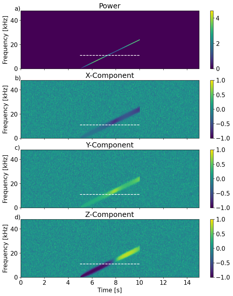
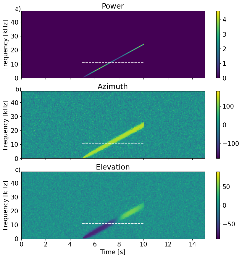
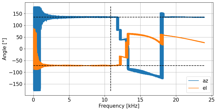
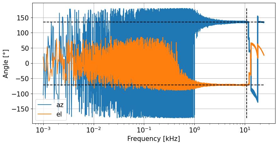
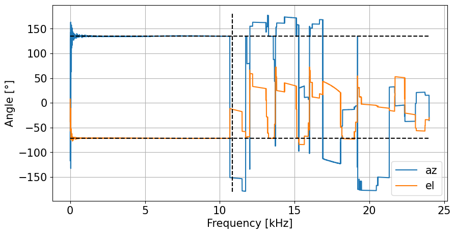
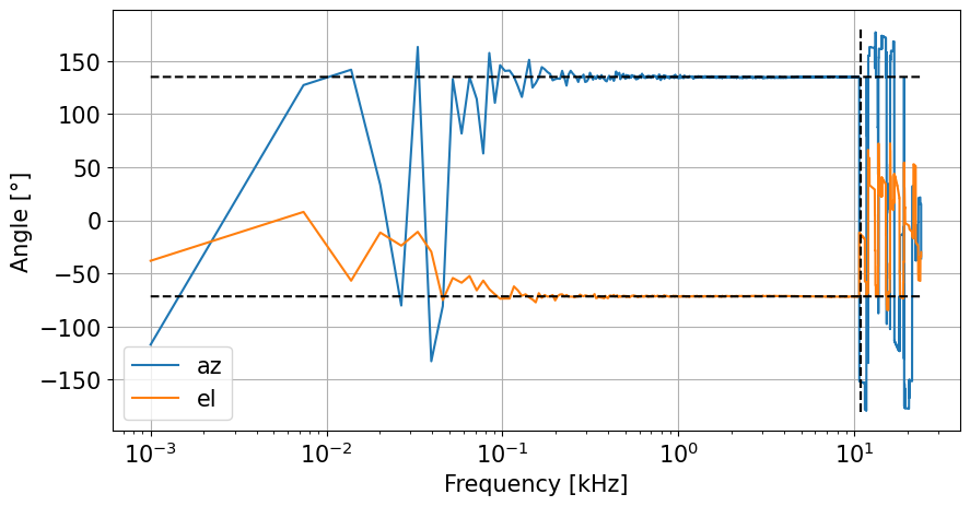
The figure shows the estimated azimuth and elevation angles as function of frequency versus time. The two horizontal dashed lines indicate the two spectral limits where phase-based operations are unique. The lower line considers all hydrophone pairs (including the 3 longer cross-diagonal ones) and the upper line corresonds to the 12 ‘normal’ hydrophone pairs.
Direction finding using phase differences#
azx,elx,t,f = bat.directionFinding(xx,DI,hsel,fs,method='Phase')

fr=f1+(f2-f1)*tt/t2
ifr=int(to*fs)+np.arange(len(fr),dtype='int')
frk=fr/1000

def Angle_plot(frx,azx,elx,Lm,scale):
    fig = plt.figure("figsize",[10,5])
    plt.plot(frx,azx,label='az')
    plt.plot(frx,elx,label='el')
    plt.plot(frx,180/np.pi*az+0*frx,'k--')
    plt.plot(frx,180/np.pi*el+0*frx,'k--')
    plt.vlines(np.min(Lm),-180,180,colors='k',linestyles='--')
    plt.vlines(np.max(Lm),-180,180,colors='k',linestyles='--')
    #plt.xlim(1e-4,24)
    plt.gca().set_xscale(scale)
    plt.legend()
    plt.grid(True)
    plt.xlabel('Frequency [kHz]')
    plt.ylabel('Angle [°]')
    plt.show()


Angle_plot(frk,azx[ifr],elx[ifr],0.75/L,'linear')
Angle_plot(frk,azx[ifr],elx[ifr],0.75/L,'log')
Direction finding using hydrophone spectrogram based cross correlation#
nh=1+int(np.ceil(np.max(L/1500*fs)))
nw=256
azx,elx,t,f=bat.directionFinding(xx,DI,hsel,fs,nw=nw,nfft=2*nw,nh=nh, method="XCORR")
#
nstep=nw//2
fx=np.zeros(ss.shape[0])
fx[:int(to*fs)]=np.nan
fx[int(to*fs):int((to+t2)*fs)]=fr
fx[int((to+t2)*fs):]=np.nan
fx1=fx[::nstep]

ifr=np.where(~np.isnan(fx1))
frk=fx1[ifr]/1000

Angle_plot(frk,azx[ifr],elx[ifr],0.75/L,'linear')
Angle_plot(frk,azx[ifr],elx[ifr],0.75/L,'log')
Direction finding using time-delay-of-arrival (tdoa) of matched filtered data#
As the signal is simulated as a linear frequency modulated time series, it is appropriate to pre-process the data using a matched filter to compress the signal into sharp transients. Using these shortened signals, standard time-delay-of arrival (tdoa) methods can be applied to obtain the direction of the sound source.
# matched filter of generated signal
zz=bat.matched_filt(sso,xx)

azx,elx,t,f,ux=bat.directionFinding(zz,DI,hsel,fs,method="TDOA_0")

print(azx,elx)
print(np.array([az,el])*180/np.pi)

tux=ux[:,0]/fs
tso=tux.mean()

n1,n2=zz.shape
n3=ux.shape[0]

plt.figure(figsize=(10,7))
plt.plot((ts-tso)*1000,zz+np.ones((n1,1))*range(n2))
plt.plot((tux-tso)*1000,ux[:,1]+np.arange(n3),'k.')
plt.xlim(-0.5,0.5)
plt.grid(True)
plt.xlabel('Time [ms]')
plt.show()
135.61281894481354 -71.35320650041636
[135.         -71.56505118]
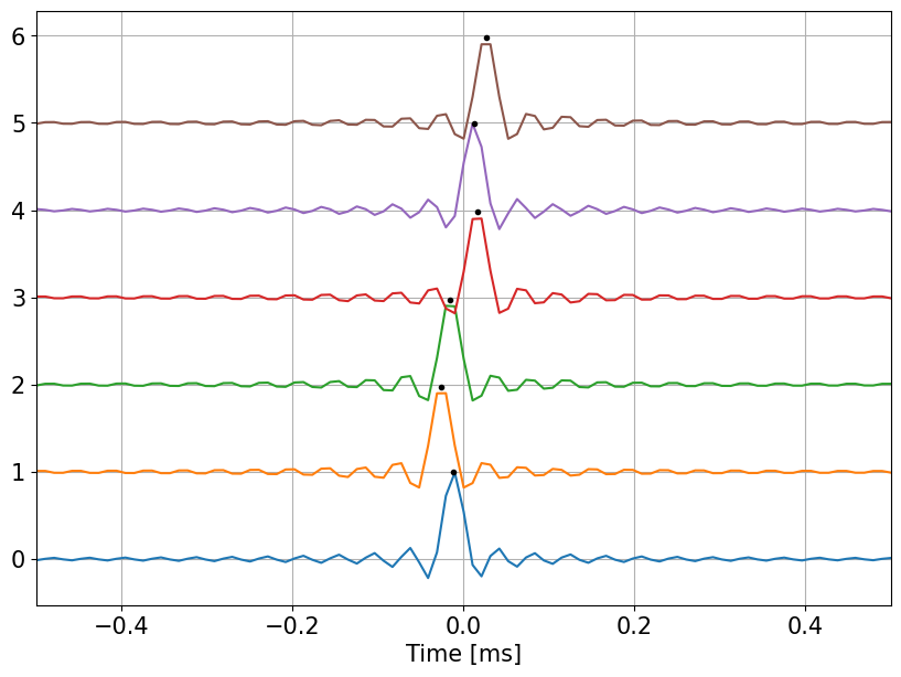
The figure shows the output of the matched filter for all hydrophones and the time delays are clearly visible. For each of the transient the time of the maximum was obtained by quadratic interpolation of 3 relevant samples. The estimated sound direction (azimuth and elevation) are very close to the simulated one.
Beamformer#
Knowing, or assuming the arrival angles of the sound, a beamformer takes the delayed time series of the array, correct for the delays and generates an average time series.
aze=azx*np.pi/180
ele=elx*np.pi/180
#
C  = bat.signal_direction(aze,ele)
DS = bat.array_delay(C,ho,sv,fs)
uu = bat.beamForm(zz,DS)
#
plt.figure(figsize=(10,7))
plt.plot((ts-tso)*1000,bat.stack(zz))
#
plt.plot((ts-tso)*1000,uu,'k')
plt.grid(True)
plt.xlim(-0.5,0.5)
plt.grid(True)
plt.xlabel('Time [ms]')
plt.show()
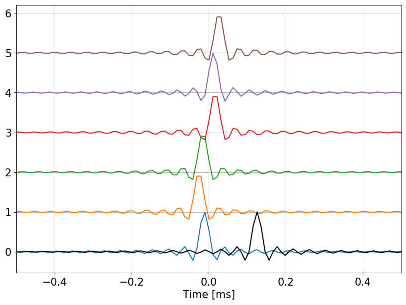
One notes that the beamformed shape corresponds to the shape of the individual signals. The observed delays are due to the fact that the delay of the sinc filters are not compenstated.