BLM_1: Basic signal spectral analysis#
The following shows some basic steps that one undertakes for signal processing.
# loading basic modules
import numpy as np
import matplotlib.pyplot as plt
Simulation of sound wave
# creation of time vector
fs = 1024
nd = int(10*fs)
tt = np.arange(nd)/fs

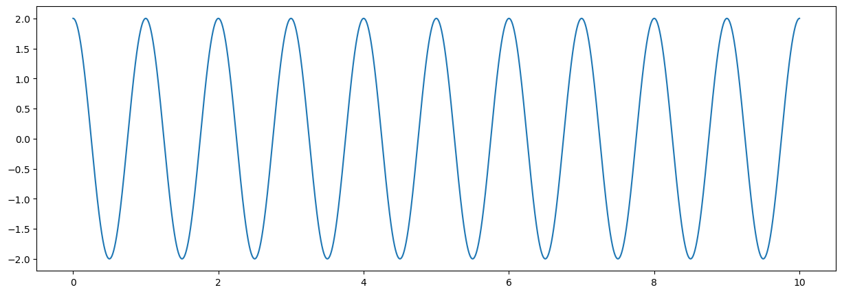
# creation of cosine signal
amp=2
xx = amp*np.cos(2*np.pi*tt)

# plot signal
fig = plt.figure("figsize",[15,5])
plt.plot(tt,xx);
plt.show();
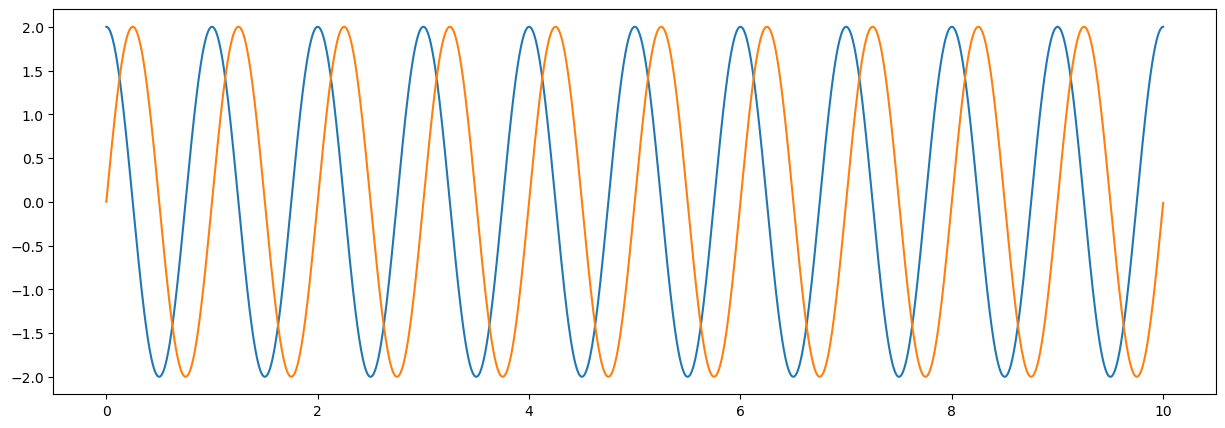
#creation of sine signal
yy = amp*np.sin(2*np.pi*tt)

fig = plt.figure("figsize",[15,5])
plt.plot(tt,xx);
plt.plot(tt,yy);
plt.show();
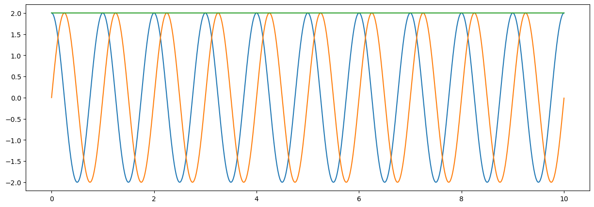
#estimation of mangnitude
zz=np.sqrt(xx**2+yy**2)

fig = plt.figure("figsize",[15,5])
plt.plot(tt,xx);
plt.plot(tt,yy);
plt.plot(tt,zz);
plt.show();
print(np.mean(xx),np.mean(yy))
print(np.mean(xx**2),np.mean(yy**2))
-8.326672684688674e-17 -1.1102230246251566e-17
1.9999999999999996 2.0
Observations#
the mean of a sinosoidal wave is zero
the mean of the signals squared is equal to the amplitude.
Complex numbers#
The following mathematical excurse is helpful for further spectral analysis
Trigonometry#
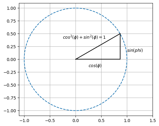
Triangle in circle
import numpy as np
import matplotlib.pyplot as plt
arg=np.arange(360)*np.pi/180
plt.plot(np.cos(arg),np.sin(arg),'--')
plt.plot([0,np.cos(np.pi/6)],[0,0],'k')
plt.plot([np.cos(np.pi/6),np.cos(np.pi/6)],[0,np.sin(np.pi/6)],'k')
plt.plot([0,np.cos(np.pi/6)],[0,np.sin(np.pi/6)],'k')
plt.grid(True)
plt.xlim(-1.1,1.5)
plt.text(1.0,0.15,"$sin(phi)$")
plt.text(0.25,-0.15,"$cos(\phi)$")
plt.text(-0.25,0.4,"$cos^2(\phi)+sin^2(\phi)=1$")
plt.gca().set_aspect('equal', adjustable='box')
plt.show()
<>:11: SyntaxWarning: invalid escape sequence '\p'
<>:12: SyntaxWarning: invalid escape sequence '\p'
<>:11: SyntaxWarning: invalid escape sequence '\p'
<>:12: SyntaxWarning: invalid escape sequence '\p'
C:\Users\zimme\AppData\Local\Temp\ipykernel_33888\1296300766.py:11: SyntaxWarning: invalid escape sequence '\p'
  plt.text(0.25,-0.15,"$cos(\phi)$")
C:\Users\zimme\AppData\Local\Temp\ipykernel_33888\1296300766.py:12: SyntaxWarning: invalid escape sequence '\p'
  plt.text(-0.25,0.4,"$cos^2(\phi)+sin^2(\phi)=1$")
Triangle
and
Pythagoras#
applied here
Problem#
Find a formula, so that sum of squares becomes constant (e.g. \(r^2\) or 1)
Hint#
We know \((a+b)*(a-b) = a^2 - b^2\), and more general \((a+c*b)*(a-c*b) = a^2 - c^2b^2\).
Solution#
Define a new symbol \(c^2 =i^2= -1\)
where \(i\) is defined such that
This way we get
Definitions#
complex number (real + i*imaginary)#
conjugate of a complex number#
absolute squared complex value by signal multiplied with its conjugate#
Alternative method#
Complex notation simplifies mathematics, but for physical phenomena only the real part is of relevance
Also from
follows
A more general expression is
so that
or equivalently
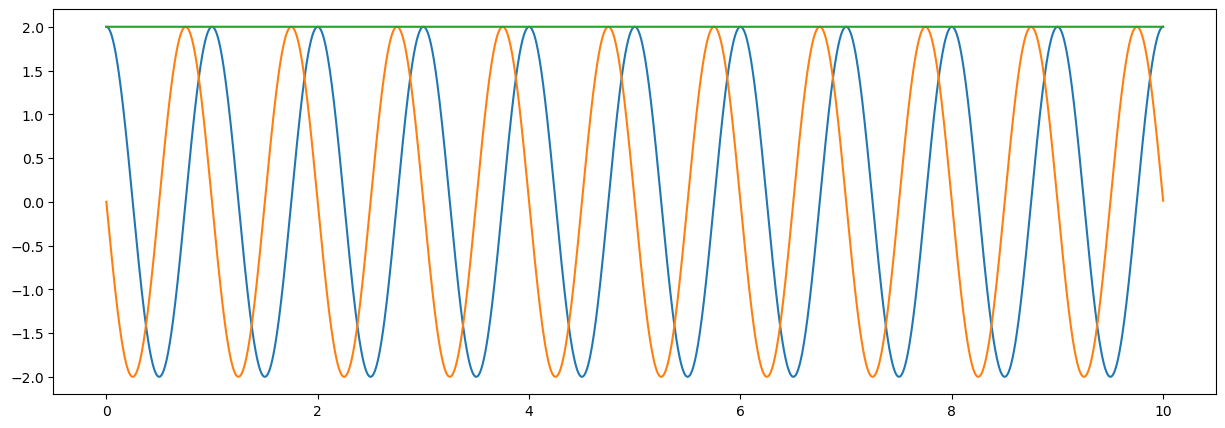
# creation of complex signal (note 1j )
xx = amp*np.exp(-2*np.pi*1j*tt)

# plot signal
fig = plt.figure("figsize",[15,5])
plt.plot(tt,np.real(xx));   # cos(xx)
plt.plot(tt,np.imag(xx));   # sin(xx)
plt.plot(tt,np.abs(xx));    # sqrt(z * conjugate(z))
plt.show();
General frequencies#
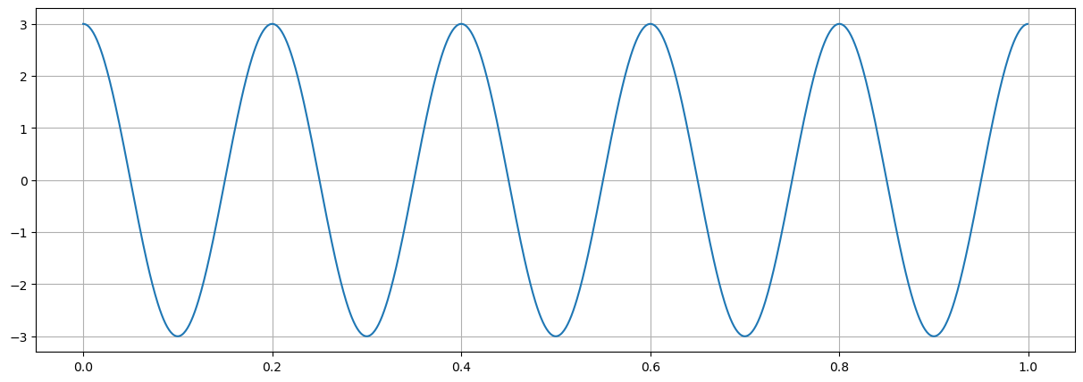
# creation of a 1 second time vector
fs = 1024 # sampling per second
nd = int(1*fs)
tt = np.arange(nd)/fs
amp=3

# signal frequency cycles/second = Hz
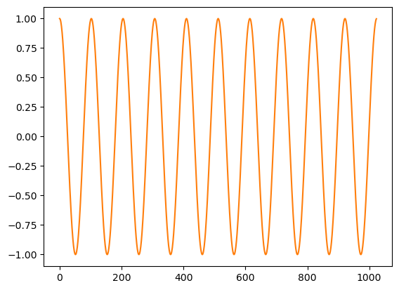
fo = 5
phi=2*np.pi*fo*tt
xx=amp*np.exp(- 1j *phi)

# plot signal
fig = plt.figure("figsize",[15,5])
plt.plot(tt,np.real(xx));
plt.grid(True)
plt.show()
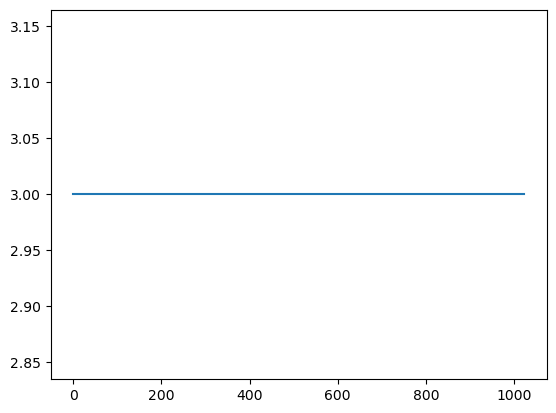
x5=amp*np.exp(- 1j * 2*np.pi*5*tt)
w5=np.exp( 1j * 2*np.pi*5*tt)
y5=x5*w5
plt.plot(np.real(y5));
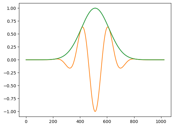
amp=np.exp(-0.5*((tt-0.5)/0.1)**2)
plt.plot(amp)
x5=amp*np.exp(- 1j * 2*np.pi*5*tt)
w5=np.exp( 1j * 2*np.pi*5*tt)
y5=x5*w5
plt.plot(np.real(x5));
plt.plot(np.abs(y5));
amp=1
fo=10
plt.plot(amp)
x5=amp*np.exp(- 1j * 2*np.pi*fo*tt)
plt.plot(np.real(x5));
plt.show()
#
plt.figure('figsize',[15,5])

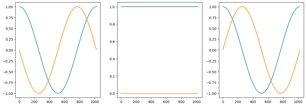
w4=np.exp( 1j * 2*np.pi*(fo-1)*tt)
y4=x5*w4
plt.subplot(131)
plt.plot(np.real(y4));
plt.plot(np.imag(y4));

w5=np.exp( 1j * 2*np.pi*fo*tt)
y5=x5*w5
plt.subplot(132)
plt.plot(np.real(y5));
plt.plot(np.imag(y5));

w6=np.exp( 1j * 2*np.pi*(fo+1)*tt)
y6=x5*w6
plt.subplot(133)
plt.plot(np.real(y6));
plt.plot(np.imag(y6));
plt.show()
Frequency analysis#
Discrete Fourier transform (DFT)#
xx=np.exp(- 1j * 2*np.pi*5*tt)

w4=np.exp(2*np.pi*1j *4*tt)
w5=np.exp(2*np.pi*1j *5*tt)
w6=np.exp(2*np.pi*1j *6*tt)

y4=np.sum(xx*w4)
y5=np.sum(xx*w5)
y6=np.sum(xx*w6)

print(y4,y5,y6)
(-2.842170943040401e-14+0j) (1024+2.958665228503174e-16j) (-8.526512829121202e-14+5.684341886080802e-14j)
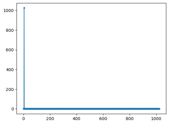
xx=np.exp(- 1j * 2*np.pi*5*tt)

# matrix of spectral analysis vectors
W=np.exp(2*np.pi*1j *np.outer(np.arange(fs),tt))

yy1=W @ xx
#yy1=np.dot(W,xx)
#yy1=W.dot(xx)
plt.plot(np.abs(yy1),'.-');
plt.show()

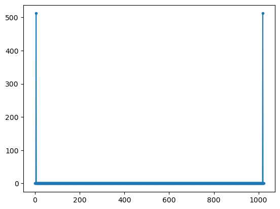
yy2=W @ np.real(xx)
plt.plot(np.abs(yy2),'.-');
plt.show()
amp=np.exp(-0.5*((tt-0.5)/0.05)**2)
fo=50
xx=amp*np.exp(- 1j * 2*np.pi*fo*tt)

# matrix of spectral analysis vectors
ff=np.arange(fs)

W=np.exp(2*np.pi*1j *np.outer(ff,tt))

yy1=W @ xx
#yy1=np.dot(W,xx)
#yy1=W.dot(xx)
plt.plot(ff,np.abs(yy1),'.-');
plt.xlim(0,100)
plt.show()

yy2=W @ np.real(xx)
plt.plot(ff,np.abs(yy2),'.-');
plt.xlim(0,100)
plt.show()
print(np.where(np.abs(yy1)>np.max(np.abs(yy1))/2))
print(np.where(np.abs(yy2)>np.max(np.abs(yy2))/2))
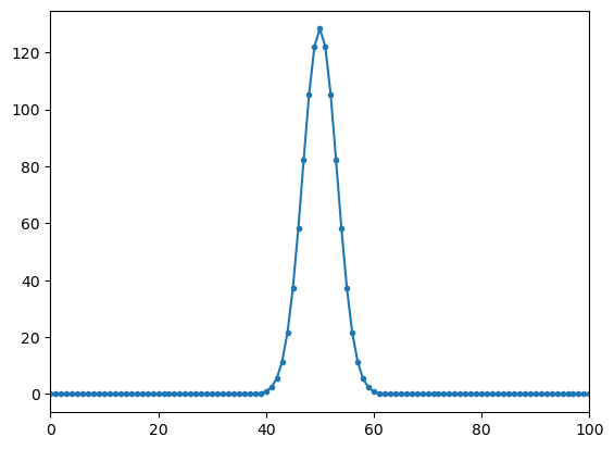
(array([47, 48, 49, 50, 51, 52, 53], dtype=int64),)
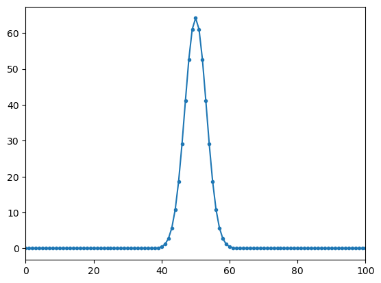
(array([ 47,  48,  49,  50,  51,  52,  53, 971, 972, 973, 974, 975, 976,
       977], dtype=int64),)
Observation#
complex signal (cos and sin) peak is at correct frequency (5) with peak amplitude that correspond to the length of the DFT
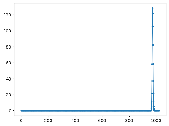
for real signals there are two peaks with half the amplitude at frequencies 5 and 1019 = (1024-5). The second peak is allso called negative frequency
the peak amplitude value of the spectrum of the complex signal is amp*length(fft)
the peak amplitude values of the spectrum of the real signal is (amp/2)*length(fft)
Fast Fourier Transform#
# generic complex to complex fft
yy=np.fft.fft(xx)

plt.plot(np.abs(yy),'.-');
plt.show()

# special real to complex fft
yy0=np.fft.rfft(np.real(xx))

plt.plot(np.abs(yy0),'.-');
plt.show()
FFT implementation#
To see how FFT is implemented (\(\exp(2\pi i nm/N)\) or \(\exp(-2\pi i nm/N)\)) we fourier transform a time series where only a single sample is set to a non-zero value (say sample 1 set to one)
In the case of a DFT we note that for a single sample
would become
taking the inverse DFT
which results to
or \(x(1)=M\) and \(x(n)=0\) for \(n \ne 1\)
#
v1 = np.exp(2*np.pi*1j*np.arange(1024)/1024)
plt.plot(np.real(v1))
plt.plot(np.imag(v1))
plt.show()

u1=np.sum(v1*np.exp(-2*np.pi*1j*np.arange(1024)/1024))
print("'DFT' peak: ", np.real(u1))
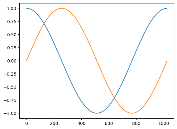
'DFT' peak: 1024.0
uu=np.zeros(1024,complex)
uu[1]=1
vv=np.fft.fft(uu)

plt.plot(np.real(vv));
plt.plot(np.imag(vv));
plt.xlabel("Frequency");
plt.show()

ww=np.fft.ifft(vv)
print("FFT peak: ",np.real(uu[1]),np.real(ww[1]))
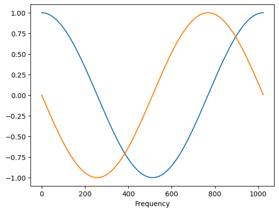
FFT peak: 1.0 1.0
Observation#
The FFT spectrum of a signle sample is \(\cos(2\pi m/N) -i \sin(2\pi m/N)\) contrary to the DFT used above that was using \(\cos(2\pi m/N) +i \sin(2\pi m/N)\) . This selection \(+i\) or \(-1\) is purely a matter of cenvention. In practical terms it means that a decision has to be made if the ‘non-real’ imaginary signal is trailing (\(+i\)) or leading \(-i\) the real signal.
As we are dealing mostly real signals and use the special rfft that only results in positive frequencies, we have not to worry about this ambiguity.
While the spectra of the FFT and DFT are equivalent (equal when ignoring the different sign of the imaginary part), the inverse FFT produces the correct original time series, while the DFT
General signal frequency#
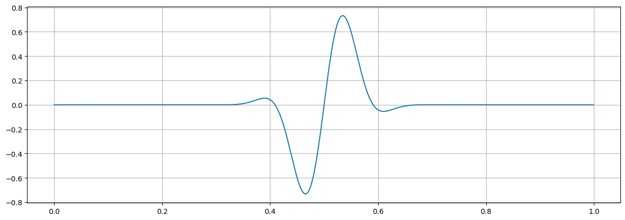
So far, the frequency was chosen to be an integer value. In the following we relax this and use a non-integer frequency, e.g.: \(f_o = 5.5\)
# signal frequency
fo = 5.5
xx=amp*np.exp(-2*np.pi*1j *fo*tt)

# plot signal
fig = plt.figure("figsize",[15,5])
plt.plot(tt,np.real(xx));
plt.grid(True)
plt.show()

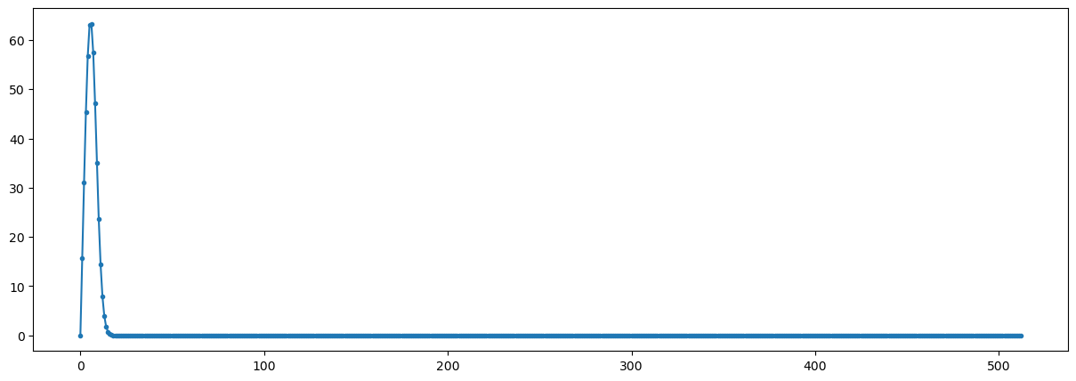
yy3=np.fft.rfft(np.real(xx))

fig = plt.figure("figsize",[15,5])
plt.plot(np.abs(yy3),'.-');
plt.show()
Observations#
Using a fractional frequency (5.5 instead of 5) different effects occur
peak is reduced to less than 700
peak is wider
most frequencies are not zero
Conclusions#
When using fractional frequencies the energy (power) of the signal is leaked to other frequencies.
Spectral leakeage#
The widening of the spectral peek occurs together with reduction in peak power and an increase for off-signal frequencies. A condition that is called spectral leakage.
One notes that the integral value of the spectral energy remains constant at (amp/2)*length(FFT)
print(np.sqrt(np.sum(np.abs(yy0)**2)),np.sqrt(np.sum(np.abs(yy3)**2)))
152.42016636452271 148.52080632743807
yy3=np.fft.rfft(np.real(xx))
xx3=np.fft.irfft(yy3)

# plot signal
fig = plt.figure("figsize",[15,5])
plt.plot(tt,np.real(xx3));
plt.grid(True)
plt.show()

Observation#
The inverse FFT of the complex spectrum generates the original time series, even if the spectrum is spead out over a wider frequency range.
Noise processing#
We now add noise to the sinusoidal signal
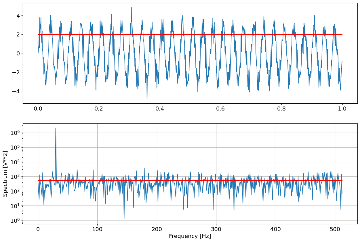
plt.rcParams.update({'font.size': 14}) # increase fontsize in figures

fs = 1024   #Hz
nfft=1024
nwin=nfft

#    Generate a 1 second test signal, a 2 Vrms sine wave at fs/8, corrupted by
#    0.001 V**2/Hz of white noise sampled at  1.024 kHz.

N = fs
time = np.arange(N) / fs

# signal description
arms=2
amp = arms*np.sqrt(2)
freq = 30

var = 0.001
noise_power = var * fs / 2
# The factor of fs/2 converts the per sample noise power (variance)
# to a noise bandwith of -1/T to 1/T (negative and positive frequencies)

xx = amp*np.sin(2*np.pi*freq*time)
rms= np.sqrt(np.mean(xx**2))

# add noise to signal
np.random.seed(1)
xx += np.random.normal(scale=np.sqrt(noise_power), size=time.shape)

print("Signal RMS : ",amp/np.sqrt(2), rms)

#
yy=np.fft.rfft(xx,nfft)
pp=np.abs(yy)**2

ff=np.arange(int(nfft/2)+1)*fs/nfft

ppmn=np.mean(pp[ff>50])
ppmx = np.max(pp)
print("Noise ",ppmn, "Peak ",ppmx)

fig = plt.figure("figure.figsize",[15,10])

plt.subplot(211)
plt.plot(time,xx)
plt.plot(time,amp/np.sqrt(2)+0*time,'r')

plt.subplot(212)
plt.semilogy(ff, pp)
plt.plot(ff,ppmn+0*ff,'r')
plt.xlabel('Frequency [Hz]')
plt.ylabel('Spectrum [V**2]')
plt.grid(True)
Signal RMS :  2.0 2.0
Noise  513.3273885838644 Peak  2073698.6295588852
print(var, 2*ppmn/(N**2))
print(arms, ppmx/(N**2))
0.001 0.0009790942928006446
2 1.9776331229771473
Observation#
To obtain noise spectrum (variance per sample), the mean value of the rfft power spectrum must be scaled by \(2/N^2\) To obtain the RMS of the signal, the peak value of the rfft power spectrum must be scaled by \(1/N^2\)
The extimates are not exactly equal as the noise is random and consequently also all extimates of noisy data are randomvariables.
Spectrum implementation#
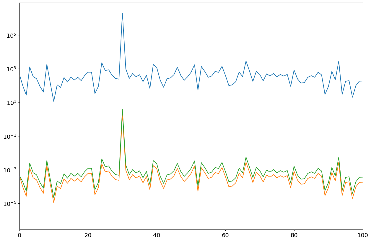
For future spectral analysis we can define the following support function that scales the power spectrum accordingly
# initial custom spectrum estimation
def mSpectrum0(xx,nfft,fs,mode=None):
    # xx: real valued time series if at least nfft samples
    # nfft: length of fft in samples
    # fs: sampling frequency
    # mode: RMS for scaling of spectral peakes to signal RMS
    #       VAR for scaling of spectral mean values to per sample variance
    #       None for power spectrum (FFT output) (Default)
    # output: P power estimates according to mode
    #         ff frequency vector
    yy=np.fft.rfft(xx[:nfft],nfft)
    ff=np.arange(int(nfft/2)+1)*fs/nfft

    pp=np.abs(yy)**2
    if mode=="RMS":
        return pp/(nfft**2), ff
    elif mode=="VAR":
        pp[1:] *= 2
        return pp/(nfft**2), ff
    else:
        return pp, ff
P1,ff = mSpectrum0(xx,nfft,fs)
P2,ff = mSpectrum0(xx,nfft,fs,"RMS")
P3,ff = mSpectrum0(xx,nfft,fs,"VAR")


fig = plt.figure("figure.figsize",[15,10])
plt.semilogy(ff,P1);
plt.semilogy(ff,P2);
plt.semilogy(ff,P3);
plt.xlim(0,100);
Windowing#
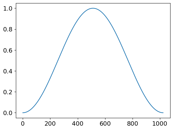
The implementation of the FFT assumes that signal is periodic. Most interesting signals are aperiodic, resulting in what is called spectral leakage. The above signal with a frequency of 5.5 is such a case.
Standard remedy is to taper the signal such that both ends of the time series are equal and very often close to zero. A typical window is the Hann window,
In the following we assume that the window length is equal to FFT length, that is we assume first NO zero padding and analyse later the case of zero padding
win=np.hanning(nwin)

plt.plot(win);
plt.show()
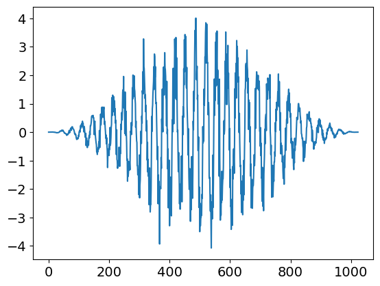
plt.plot(xx*win);
plt.show()
Observations#
Windowing reduces
the influences of initial and final data
the effective length of the data
Conclusions#
one should expect that
the RMS value of the signal is modified
the noise variance is modified
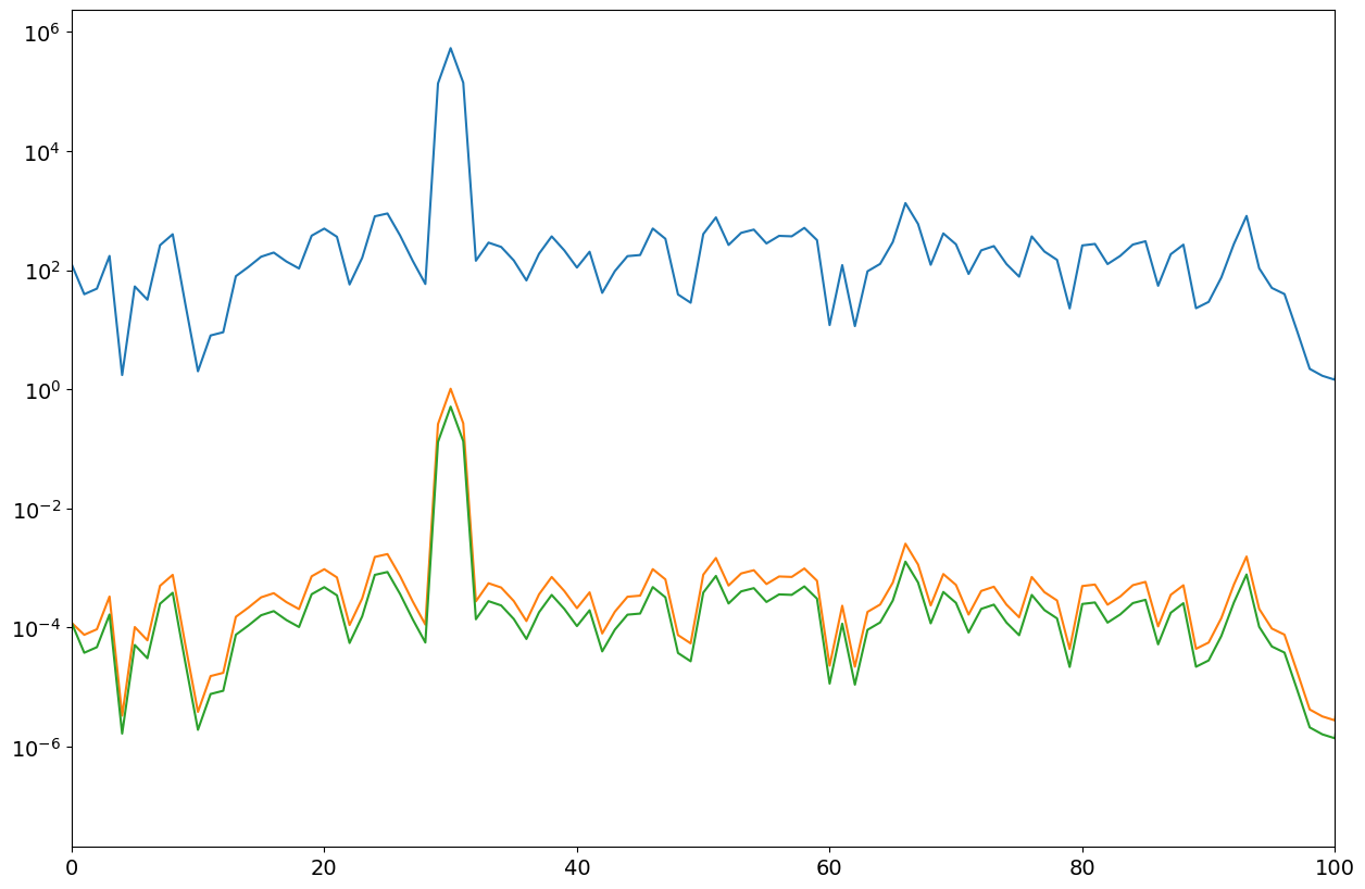
P11,ff = mSpectrum0(xx*win,nfft,fs)
P12,ff = mSpectrum0(xx*win,nfft,fs,"VAR") # for noise
P13,ff = mSpectrum0(xx*win,nfft,fs,"RMS") # for signal


fig = plt.figure("figure.figsize",[15,10])
plt.semilogy(ff,P11);
plt.semilogy(ff,P12);
plt.semilogy(ff,P13);
plt.xlim(0,100)

print(var, np.mean(P12[50:]))
print(arms, np.max(P13))
0.001 0.00039303184120769764
2 0.5095595110138033
Observation#
Both, the RMS estimate (peak value) and the per sample Var value (noise) are not correct. The obtained values are too low due to the windowing influence. This can be corrected by considering the window shape.
print(np.mean(win*win))
print(np.mean(win))

print(var, np.mean(P12[50:])/np.mean(win*win))
print(arms, np.max(P13)/win.mean()**2)
0.3746337890625
0.49951171875
0.001 0.0010491094308157248
2 2.0422248167831363
# updated custom spectrum estimation
def mSpectrum1(xx,win,fs,mode=None):
    # xx: real valued time series if at least nfft samples
    # nfft: length of fft in samples
    # fs: sampling frequency
    # mode: RMS for scaling of spectral peakes to signal RMS
    #       VAR for scaling of spectral mean values to per sample variance
    #       None for power spectrum (FFT output) (Default)
    # output: P power estimates according to mode
    #         ff frequency vector
    nwin=len(win)
    nfft=nwin
    yy=np.fft.rfft(xx[:nwin]*win,nfft)
    ff=np.arange(int(nfft/2)+1)*fs/nfft

    pp=np.abs(yy)**2
    if mode=="RMS":
        return pp/win.sum()**2, ff
    elif mode=="VAR":
        pp[1:] *=2
        return pp/(nwin*(win*win).sum()), ff
    else:
        return pp, ff
P21,ff = mSpectrum1(xx,win,fs)
P22,ff = mSpectrum1(xx,win,fs,"VAR")
P23,ff = mSpectrum1(xx,win,fs,"RMS")


fig = plt.figure("figure.figsize",[15,10])
plt.semilogy(ff,P21);
plt.semilogy(ff,P22);
plt.semilogy(ff,P23);
plt.xlim(0,100)

# test estimates
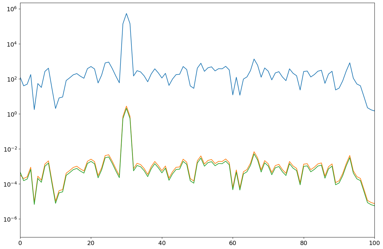
print(var, np.mean(P22[50:]))
print(arms, np.max(P23))
0.001 0.0010491094308157246
2 2.0422248167831363
Observations#
The general scaling functions of spectras are
RMS estimation:
1/win.sum()**2VAR estimation:
2/(nwin*(win*win).sum()), whereby the factor 2 is only for nonzero frequencies
For rectangular windows (that is no windows) we have win.sum()=nwin and (win*win).sum()=nwin
Power spectral density (PSD)#
The VAR estimation provides the per sample noise variance expressed in V^2/sample . To obtain the PSD that typically is expressed in V^2/Hz one needs to consider the spectral binwidth in terms of the sampling frequency \(f_s\).
Binwidth in Hz is for \(N_{fft}= N_{win}\) given by
and therfore the PSD related scaling of the spectra
PSD estimation:
2/(nwin*(win*win).sum())*nwin/fsor2/(fs*(win*win).sum())
Zero padding#
So far, we assumed that the length of the fft is equal to the length of the window. In the following we allow the fft length to be longer than the window length, wherby the added samples are kept at zero (zero padding).
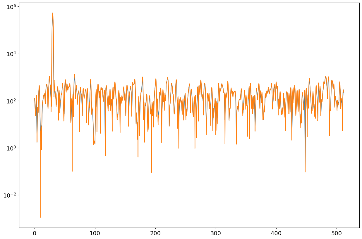
# case 1
nfft1=nwin
uu=xx[:nwin]*win
yy1=np.fft.rfft(uu,nfft1)
ff1=np.arange(int(nfft1/2)+1)*fs/nfft1

pp1=np.abs(yy1)**2

# case 2
nfft2=4*nwin
uu=np.zeros(nfft2)
uu[:nwin] = xx[:nwin]*win
yy2=np.fft.rfft(uu,nfft2)
ff2=np.arange(int(nfft2/2)+1)*fs/nfft2

pp2=np.abs(yy2)**2

fig = plt.figure("figure.figsize",[15,10])
plt.semilogy(ff1,pp1);
plt.semilogy(ff2,pp2);

print(np.max(pp1),np.max(pp2))
print(np.mean(pp1[ff1>40]),np.mean(pp2[ff2>40]))
534311.8738208098 534311.8738208096
205.5119088000577 205.5145016630521
Observations#
We note that the unscaled spectra estimates do not vary when adding zeros to the data before FFT (zero padding). All what is changing is the number of frequency bins to cover the whole spectrum and consequently, zero padded FFTs are also called interpolationg FFT.
One should expect that scaling for the RMS estimate (peak of spectrogram) does not depend on length of zero padded FFT but only on length of window
Open question: does zero padding change the estimate of the PSD?#
The PSD is given as the time averaged spectral energy
or for discrete sampling
where \(N\) is the number of samples of the signal and \(\Delta t\) is the sampling interval, i.e. \(N\Delta t=T\) is the length of the signal in seconds and \(n\Delta t\) is the time when the n-th samples was measured.
The quantity \(P(f)\) is really a time averaged signal energy
Assume zero padding from \(N\) to \(K>N\), the sum does not change as \(x(n)=0\) for all \(n>N\), but the frequency interpretation does:
Assume \(f_k =k(f_s/K)\) for \(k=0,1, ...,K-1\) with \(f_s = 1/\Delta t\)
The PSD is independent of the DFT size K, but it only depends on the number of time domain samples N
Comment#
Zero padding is only useful if one is interested in the interpolating aspect of the zero-padded FFT, e.g. for RMS estimates of tonal signals. For broadband PSD estimation zero-padded FFT seems of little advantage.
Custom Spectrum implementation#
# custom spectrum estimation
def mSpectrum(xx,win,fs,nfft,mode=None):
    # xx: real valued time series if at least nfft samples
    # nfft: length of fft in samples
    # fs: sampling frequency
    # mode: RMS for scaling of spectral peakes to signal RMS
    #       VAR for scaling of spectral mean values to per sample variance
    #       PSD for scaling of power spectral density to (v^2/Hz)
    #       None for power spectrum (FFT output) (Default)
    # output: P power estimates according to mode
    #         ff frequency vector
    nwin=len(win)
    if nfft<nwin: nfft=nwin # force nfft to be at least window length
    nfft=int(2**np.ceil(np.log2(nfft))) # increase nfft to next power of 2
    #
    # copy data to working buffer zero-pad if required
    uu=np.zeros(nfft)
    uu[:nwin]=xx[:nwin]*win

    yy=np.fft.rfft(uu,nfft)
    ff=np.arange(int(nfft/2)+1)*fs/nfft

    pp=np.abs(yy)**2
    if mode=="RMS":
        return pp/win.sum()**2, ff
    elif mode=="VAR":
        pp[1:] *=2
        return pp/(nwin*(win*win).sum()), ff
    elif mode=="PSD":
        pp[1:] *=2
        return pp/(fs*(win*win).sum()), ff
    else:
        return pp, ff
# case 1
nfft1=nwin
# case 2
nfft2=4*nwin

#----------------------------------------------
pp1,ff1=mSpectrum(xx,win,fs,nfft1,"RMS")
pp2,ff2=mSpectrum(xx,win,fs,nfft2,"RMS")

fig = plt.figure("figure.figsize",[15,10])
plt.semilogy(ff1,pp1);
plt.semilogy(ff2,pp2);
plt.show()

print("RMS: ",np.max(pp1),np.max(pp2))

#----------------------------------------------
pp1,ff1=mSpectrum(xx,win,fs,nfft1,"PSD")
pp2,ff2=mSpectrum(xx,win,fs,nfft2,"PSD")

fig = plt.figure("figure.figsize",[15,10])
plt.semilogy(ff1,pp1);
plt.semilogy(ff2,pp2);
plt.show()

print("PSD: ", np.mean(pp1[ff1>40]),np.mean(pp2[ff2>40]))
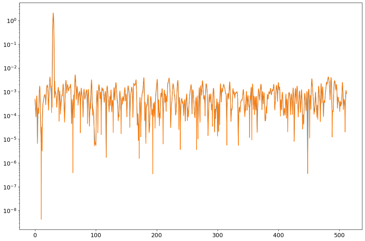
RMS: 2.0422248167831363 2.042224816783136

PSD: 0.0010463094086024442 0.0010463226094770898
Comments#
For a complex sinusoidal signal the Python FFT gives a negative frequency (fs-5 = 1019)
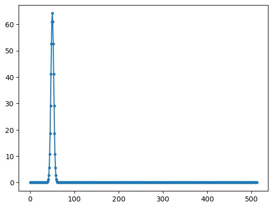
a special version of the FFT call rfft gives only the positive frequencies (x-axis only up to fs/2 and not fs)